|
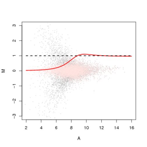
| Figure 5.11: The variance--bias trade-off and VSN 's property as a shrinkage estimator . Shown is an MA-plot of the kidney data. Dark dots correspond to the naive log_2-ratio , as in Equation~( eq:ratio ), and light dots to the glog_2-ratio , as in Equation~( eq:glogratio ). The two samples that are compared in these data were taken from immediately adjacent pieces of tissue, so most of the genes are not differentially expressed and have a true log fold-change of 0. Accordingly, both the naive log_2-ratio and the glog_2 -ratio are distributed around zero. However, for the naive log_2-ratio , the width of the distribution is bigger for small values of the average intensity A , as can be seen from the ``rocket shape'' of the distribution. For the glog_2-ratio , the width is approximately constant throughout the range of A . (The visually apparent widening in the intermediate range around A=8 is solely due to the larger density of data points; see Figure~ vsn-meanSdCCl4 for a visualization that avoids this artifact.) The lines in this plot are drawn between a set of 29 data points which we have artificially ``spiked in'' to have a naive log_2-ratio of log_2(2)=1, at various values of A. This demonstrates the shrinkage effect of VSN : for low intensity data, the glog_2-ratio (solid line), as an estimator of fold-change , shrinks towards zero, but maintains a constant small variance. In contrast, the naive log_2-ratio (dashed line) is unbiased, but its variance increases for low average intensities A . |