---
title: "Structure and content of RAVmodel"
author: "Sehyun Oh"
date: "`r format(Sys.time(), '%B %d, %Y')`"
vignette: >
%\VignetteEngine{knitr::rmarkdown}
%\VignetteIndexEntry{Introduction on RAVmodel}
%\VignetteEncoding{UTF-8}
output:
BiocStyle::html_document:
number_sections: yes
toc: yes
toc_depth: 4
---
```{r setup, include = FALSE}
knitr::opts_chunk$set(
collapse = TRUE, comment = "#>"
)
```
# Setup
## Install and load package
```{r eval = FALSE}
if (!require("BiocManager"))
install.packages("BiocManager")
BiocManager::install("GenomicSuperSignature")
```
```{r results="hide", message=FALSE, warning=FALSE}
library(GenomicSuperSignature)
```
## Download RAVmodel
You can download GenomicSuperSignature from Google Cloud bucket using
`GenomicSuperSignature::getModel` function. Currently available models are
built from top 20 PCs of 536 studies (containing 44,890 samples) containing
13,934 common genes from each of 536 study's top 90% varying genes based on
their study-level standard deviation. There are two versions of this RAVmodel
annotated with different gene sets for GSEA: MSigDB C2 (`C2`) and three
priors from PLIER package (`PLIERpriors`). In this vignette, we are showing
the `C2` annotated model.
Note that the first interactive run of this code, you will be asked to allow
R to create a cache directory. The model file will be stored there and
subsequent calls to `getModel` will read from the cache.
```{r load_model}
RAVmodel <- getModel("C2", load=TRUE)
```
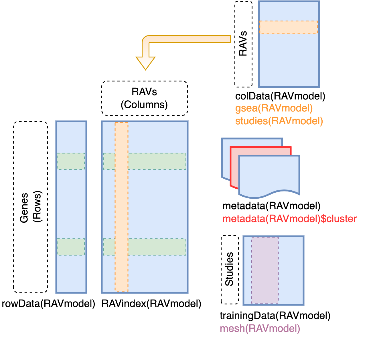
# Content of RAVmodel
`RAVindex` is a matrix containing genes in rows and RAVs in columns. `colData`
slot provides the information on each RAVs, such as GSEA annotation and
studies involved in each cluster. `metadata` slot stores model construction
information. `trainingData` slot contains the information on individual
studies in training dataset, such as MeSH terms assigned to each study.
```{r}
RAVmodel
```
 ## RAVindex
*R*eplicable *A*xis of *V*ariation (RAV) index is the main component of
GenomicSuperSignature. It serves as an index connecting new datasets and the
existing database. You can access it through `GenomicSuperSignature::RAVindex`
(equivalent of `SummarizedExperiment::assay`). Rows are genes and columns are
RAVs.
Here, RAVmodel consists of 13,934 genes and 4,764 RAVs.
```{r}
class(RAVindex(RAVmodel))
dim(RAVindex(RAVmodel))
RAVindex(RAVmodel)[1:4, 1:4]
```
## Metadata for RAVmodel
Metadata slot of RAVmodel contains information related to the model building.
```{r}
names(metadata(RAVmodel))
```
* `cluster` : cluster membership of each PCs from the training dataset
* `size` : an integer vector with the length of clusters, containing the number
of PCs in each cluster
* `k` : the number of all clusters in the given RAVmodel
* `n` : the number of top PCs kept from each study in the training dataset
* `geneSets` : the name of gene sets used for GSEA annotation
* `MeSH_freq` : the frequency of MeSH terms associated with the training
dataset. MeSH terms like 'Humans' and 'RNA-seq' are top ranked (which is very
expected) because the training dataset of this model is Human RNA sequencing
data.
* `updateNote` : a brief note on the given model's specification
* `version` : the version of the given model
```{r}
head(metadata(RAVmodel)$cluster)
head(metadata(RAVmodel)$size)
metadata(RAVmodel)$k
metadata(RAVmodel)$n
geneSets(RAVmodel)
head(metadata(RAVmodel)$MeSH_freq)
updateNote(RAVmodel)
metadata(RAVmodel)$version
```
## Studies in each RAV
You can find which studies are in each cluster using `studies` method. Output is
a list with the length of clusters, where each element is a character vector
containing the name of studies in each cluster.
```{r}
length(studies(RAVmodel))
studies(RAVmodel)[1:3]
```
You can check which PC from different studies are in RAVs using `PCinRAV`.
```{r}
PCinRAV(RAVmodel, 2)
```
## Silhouette width for each RAV
Silhouette width ranges from -1 to 1 for each cluster. Typically, it is
interpreted as follows:
- Values close to 1 suggest that the observation is well matched to the
assigned cluster
- Values close to 0 suggest that the observation is borderline matched
between two clusters
- Values close to -1 suggest that the observations may be assigned to the
wrong cluster
For RAVmodel, the average silhouette width of each cluster is a quality control
measure and suggested as a secondary reference to choose proper RAVs,
following validation score.
```{r}
x <- silhouetteWidth(RAVmodel)
head(x) # average silhouette width of the first 6 RAVs
```
## GSEA on each RAV
Pre-processed GSEA results on each RAV are stored in RAVmodel and can be
accessed through `gsea` function.
```{r}
class(gsea(RAVmodel))
class(gsea(RAVmodel)[[1]])
length(gsea(RAVmodel))
gsea(RAVmodel)[1]
```
## MeSH terms for each study
You can find MeSH terms associated with each study using `mesh` method.
Output is a list with the length of studies used for training. Each element of
this output list is a data frame containing the assigned MeSH terms and the
detail of them. The last column `bagOfWords` is the frequency of the MeSH term
in the whole training dataset.
```{r}
length(mesh(RAVmodel))
mesh(RAVmodel)[1]
```
## PCA summary for each study
PCA summary of each study can be accessed through `PCAsummary` method. Output
is a list with the length of studies, where each element is a matrix containing
PCA summary results: standard deviation (SD), variance explained by each PC
(Variance), and the cumulative variance explained (Cumulative).
```{r}
length(PCAsummary(RAVmodel))
PCAsummary(RAVmodel)[1]
```
# Session Info
## RAVindex
*R*eplicable *A*xis of *V*ariation (RAV) index is the main component of
GenomicSuperSignature. It serves as an index connecting new datasets and the
existing database. You can access it through `GenomicSuperSignature::RAVindex`
(equivalent of `SummarizedExperiment::assay`). Rows are genes and columns are
RAVs.
Here, RAVmodel consists of 13,934 genes and 4,764 RAVs.
```{r}
class(RAVindex(RAVmodel))
dim(RAVindex(RAVmodel))
RAVindex(RAVmodel)[1:4, 1:4]
```
## Metadata for RAVmodel
Metadata slot of RAVmodel contains information related to the model building.
```{r}
names(metadata(RAVmodel))
```
* `cluster` : cluster membership of each PCs from the training dataset
* `size` : an integer vector with the length of clusters, containing the number
of PCs in each cluster
* `k` : the number of all clusters in the given RAVmodel
* `n` : the number of top PCs kept from each study in the training dataset
* `geneSets` : the name of gene sets used for GSEA annotation
* `MeSH_freq` : the frequency of MeSH terms associated with the training
dataset. MeSH terms like 'Humans' and 'RNA-seq' are top ranked (which is very
expected) because the training dataset of this model is Human RNA sequencing
data.
* `updateNote` : a brief note on the given model's specification
* `version` : the version of the given model
```{r}
head(metadata(RAVmodel)$cluster)
head(metadata(RAVmodel)$size)
metadata(RAVmodel)$k
metadata(RAVmodel)$n
geneSets(RAVmodel)
head(metadata(RAVmodel)$MeSH_freq)
updateNote(RAVmodel)
metadata(RAVmodel)$version
```
## Studies in each RAV
You can find which studies are in each cluster using `studies` method. Output is
a list with the length of clusters, where each element is a character vector
containing the name of studies in each cluster.
```{r}
length(studies(RAVmodel))
studies(RAVmodel)[1:3]
```
You can check which PC from different studies are in RAVs using `PCinRAV`.
```{r}
PCinRAV(RAVmodel, 2)
```
## Silhouette width for each RAV
Silhouette width ranges from -1 to 1 for each cluster. Typically, it is
interpreted as follows:
- Values close to 1 suggest that the observation is well matched to the
assigned cluster
- Values close to 0 suggest that the observation is borderline matched
between two clusters
- Values close to -1 suggest that the observations may be assigned to the
wrong cluster
For RAVmodel, the average silhouette width of each cluster is a quality control
measure and suggested as a secondary reference to choose proper RAVs,
following validation score.
```{r}
x <- silhouetteWidth(RAVmodel)
head(x) # average silhouette width of the first 6 RAVs
```
## GSEA on each RAV
Pre-processed GSEA results on each RAV are stored in RAVmodel and can be
accessed through `gsea` function.
```{r}
class(gsea(RAVmodel))
class(gsea(RAVmodel)[[1]])
length(gsea(RAVmodel))
gsea(RAVmodel)[1]
```
## MeSH terms for each study
You can find MeSH terms associated with each study using `mesh` method.
Output is a list with the length of studies used for training. Each element of
this output list is a data frame containing the assigned MeSH terms and the
detail of them. The last column `bagOfWords` is the frequency of the MeSH term
in the whole training dataset.
```{r}
length(mesh(RAVmodel))
mesh(RAVmodel)[1]
```
## PCA summary for each study
PCA summary of each study can be accessed through `PCAsummary` method. Output
is a list with the length of studies, where each element is a matrix containing
PCA summary results: standard deviation (SD), variance explained by each PC
(Variance), and the cumulative variance explained (Cumulative).
```{r}
length(PCAsummary(RAVmodel))
PCAsummary(RAVmodel)[1]
```
# Session Info
```{r}
sessionInfo()
```