---
title: 'statTarget'
author: "Hemi Luan"
date: "Modified: 5 Jan 2017. Compiled: `r format(Sys.Date(), '%d %b %Y')`"
output:
BiocStyle::html_document:
toc: true
vignette: >
%\VignetteIndexEntry{statTargetIntroduction}
%\VignetteEngine{knitr::rmarkdown}
\usepackage[utf8]{inputenc}
---
```{r style, echo = FALSE, results = 'asis'}
BiocStyle::markdown()
```
```{r, echo = FALSE}
knitr::opts_chunk$set(collapse = TRUE, comment = "#>")
```
# Background
`Quality Control (QC)` has been considered as an essential step in the
metabolomics platform for high reproducibility and accuracy of data.
The repetitive use of the same QC samples is more and more accepted for
correcting the signal drift during the sequence of MS run order,
especially beneficial to improve the quality of data in multi-block
experiments of `large-scale metabolomic study`. statTarget is an easy use tool
to provide a graphical user interface for `quality control based
signal shift correction`, integration of metabolomic data from `multi-batch
experiments`, and comprehensive statistic analysis in
non-targeted or targeted metabolomics.
This document is intended to guide the user to use `statTargetGUI` to
perform metabolomic data analysis. Note that this document will
not describe the inner workings
of `statTarget algorithm`.
## System requirements
Dependent on R (>= 3.3.0)
## Opening the GUI
Load the package with biocLite():
```{r subsetting-GTuples4, eval = TRUE, echo = TRUE}
source("https://bioconductor.org/biocLite.R")
biocLite("statTarget")
```
For mac PC, the package statTargetGUI requires X11 support (XQuartz).
Download it from https://www.xquartz.org.
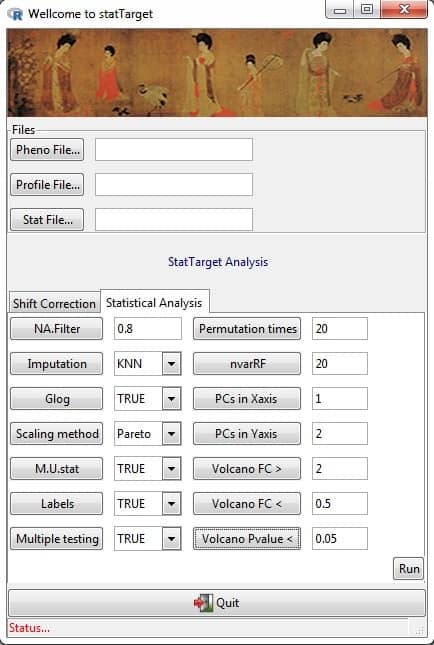
# GUI overview
An easy to use tool providing a graphical user interface (Figure 1) for
quality control based signal correction, integration of metabolomic
data from multiple batches, and comprehensive statistic analysis
for non-targeted and targeted approaches.
(URL: https://github.com/13479776/statTarget)
## What does statTarget offer statistically
The main GUI of statTarget has two basic sections. The first section
is Shift Correction. It includes quality control-based robust LOESS signal
correction (QC-RLSC) that is a widely accepted method for quality control
based signal correction and integration of metabolomic data from multiple
analytical batches (Dunn WB., et al. 2011; Luan H., et al. 2015). The second
section is Statistical Analysis. It provides comprehensively computational
and statistical methods that are commonly applied to analyze metabolomics data,
and offers multiple results for biomarker discovery.
 `Section 1 - Shift Correction` provide QC-RLSC algorithm
that fit the QC data,
and each metabolites in the true sample will be normalized to the QC sample.
To avoid overfitting of the observed data, LOESS based generalised
cross-validation (GCV) would be automatically applied,
when the QCspan was set at 0.
`Section 2 - Statistical Analysis` provide features including Data
preprocessing,
Data descriptions, Multivariate statistics analysis and Univariate analysis.
Data preprocessing : 80-precent rule, glog transformation, KNN imputation,
Median imputation and Minimum values imputation.
Data descriptions : Mean value, Median value, Sum, Quartile, Standard
derivatives, etc.
Multivariate statistics analysis : PCA, PLSDA, VIP, Random forest.
Univariate analysis : Welch's T-test, Shapiro-Wilk normality test and
Mann-Whitney test.
Biomarkers analysis: ROC, Odd ratio.
## Running Shift Correction from the GUI
`Pheno File`
Meta information includes the Sample name, class, batch and order.
Do not change the name of each column.
(a) Class: The QC should be labeled as NA.
(b) Order : Injection sequence.
(c) Batch: The analysis blocks or batches with ordinal number,e.g., 1,2,3,....
(d) Sample name should be consistent in Pheno file and Profile file.
(See the example data)
`Profile File`
Expression data includes the sample name and expression
data.(See the example data)
`NA.Filter`
NA.Filter: Removing peaks with more than 80 percent of missing values
(NA or 0) in each group. (Default: 0.8)
`QCspan`
The smoothing parameter which controls the bias-variance tradeoff.
The common range of QCspan value is from 0.2 to 0.75. If you choose
a span that is too small then there will be a large variance.
If the span is too large, a large bias will be produced.
The default value of QCspan is set at '0', the generalised
cross-validation will be performed for choosing a good value,
avoiding overfitting of the observed data. (Default: 0)
`degree`
Lets you specify local constant regression (i.e.,
the Nadaraya-Watson estimator, degree=0),
local linear regression (degree=1), or local polynomial fits (degree=2).
(Default: 2)
`Imputation`
Imputation: The parameter for imputation method.(i.e.,
nearest neighbor averaging, "KNN"; minimum values for imputed variables,
"min"; median values for imputed variables (Group dependent) "median".
(Default: KNN)
## Running Statistical Analysis from the GUI
`Stat File`
Expression data includes the sample name, group, and expression data.
`NA.Filter`
Removing peaks with more than 80 percent of missing values (NA or 0)
in each group. (Default: 0.8)
`Imputation`
The parameter for imputation method.(i.e., nearest neighbor averaging,
"KNN"; minimum values for imputed variables, "min";
median values for imputed variables (Group dependent) "median". (Default: KNN)
`Glog`
Generalised logarithm (glog) transformation for Variance stabilization
(Default: TRUE)
`Scaling Method`
Scaling method before statistic analysis (PCA or PLS).
Pareto can be used for specifying the Pareto scaling.
Auto can be used for specifying the Auto scaling (or unit variance scaling).
Vast can be used for specifying the vast scaling. Range can be used for
specifying the Range scaling. (Default: Pareto)
`M.U.Stat`
Multiple statistical analysis and univariate analysis (Default: TRUE)
`Permutation times`
The number of random permutation times for PLS-DA model (Default: 20)
`PCs`
PCs in the Xaxis or Yaxis: Principal components in
PCA-PLS model for the x or y-axis (Default: 1 and 2)
`nvarRF`
The number of variables in Gini plot of Randomforest model (=< 100).
(Default: 20)
`Labels`
To show the name of sample in the Score plot. (Default: TRUE)
`Multiple testing`
This multiple testing correction via false discovery rate (FDR)
estimation with Benjamini-Hochberg method. The false discovery rate
for conceptualizing the rate of type I errors in null hypothesis
testing when conducting multiple comparisons. (Default: TRUE)
`Volcano FC`
The up or down -regulated metabolites using Fold Changes cut off
values in the Volcano plot. (Default: > 2 or < 1.5)
`Volcano Pvalue`
The significance level for metabolites in the Volcano plot.(Default: 0.05)
# Investigating the results
Download the [statTarget tutorial](https://github.com/13479776/Picture/raw/master/work%20flow.pptx) and [example data](https://github.com/13479776/Picture/raw/master/Data_example.zip) .
Once data files have been analysed it is time to investigate them.
Please get this info. through the GitHub page.
(URL: https://github.com/13479776/statTarget)
## Results of Shift Correction (ShiftCor)
- __The output file: __
```
statTarget -- shiftCor
-- After_shiftCor # The corrected results including the loplot using statTarget
-- Before_shiftCor # The raw results using statTarget
-- RSDresult # The RSD analysis
```
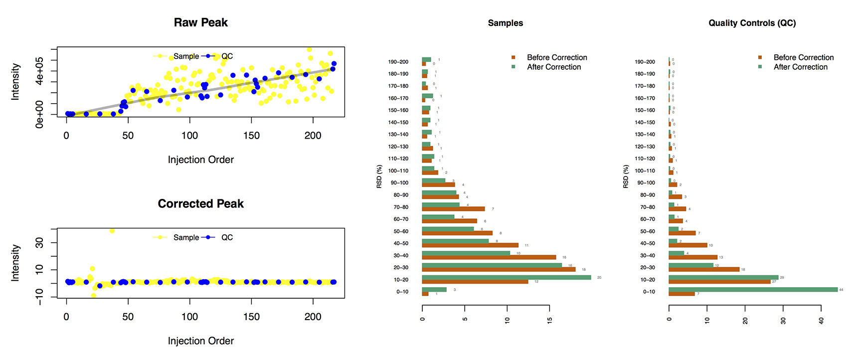
- **The Figures:**
Loplot (left): the visible Figure of QC-RLS correction for each peak.
The RSD distribution (right):
The relative standard deviation of peaks in the samples and QCs
`Section 1 - Shift Correction` provide QC-RLSC algorithm
that fit the QC data,
and each metabolites in the true sample will be normalized to the QC sample.
To avoid overfitting of the observed data, LOESS based generalised
cross-validation (GCV) would be automatically applied,
when the QCspan was set at 0.
`Section 2 - Statistical Analysis` provide features including Data
preprocessing,
Data descriptions, Multivariate statistics analysis and Univariate analysis.
Data preprocessing : 80-precent rule, glog transformation, KNN imputation,
Median imputation and Minimum values imputation.
Data descriptions : Mean value, Median value, Sum, Quartile, Standard
derivatives, etc.
Multivariate statistics analysis : PCA, PLSDA, VIP, Random forest.
Univariate analysis : Welch's T-test, Shapiro-Wilk normality test and
Mann-Whitney test.
Biomarkers analysis: ROC, Odd ratio.
## Running Shift Correction from the GUI
`Pheno File`
Meta information includes the Sample name, class, batch and order.
Do not change the name of each column.
(a) Class: The QC should be labeled as NA.
(b) Order : Injection sequence.
(c) Batch: The analysis blocks or batches with ordinal number,e.g., 1,2,3,....
(d) Sample name should be consistent in Pheno file and Profile file.
(See the example data)
`Profile File`
Expression data includes the sample name and expression
data.(See the example data)
`NA.Filter`
NA.Filter: Removing peaks with more than 80 percent of missing values
(NA or 0) in each group. (Default: 0.8)
`QCspan`
The smoothing parameter which controls the bias-variance tradeoff.
The common range of QCspan value is from 0.2 to 0.75. If you choose
a span that is too small then there will be a large variance.
If the span is too large, a large bias will be produced.
The default value of QCspan is set at '0', the generalised
cross-validation will be performed for choosing a good value,
avoiding overfitting of the observed data. (Default: 0)
`degree`
Lets you specify local constant regression (i.e.,
the Nadaraya-Watson estimator, degree=0),
local linear regression (degree=1), or local polynomial fits (degree=2).
(Default: 2)
`Imputation`
Imputation: The parameter for imputation method.(i.e.,
nearest neighbor averaging, "KNN"; minimum values for imputed variables,
"min"; median values for imputed variables (Group dependent) "median".
(Default: KNN)
## Running Statistical Analysis from the GUI
`Stat File`
Expression data includes the sample name, group, and expression data.
`NA.Filter`
Removing peaks with more than 80 percent of missing values (NA or 0)
in each group. (Default: 0.8)
`Imputation`
The parameter for imputation method.(i.e., nearest neighbor averaging,
"KNN"; minimum values for imputed variables, "min";
median values for imputed variables (Group dependent) "median". (Default: KNN)
`Glog`
Generalised logarithm (glog) transformation for Variance stabilization
(Default: TRUE)
`Scaling Method`
Scaling method before statistic analysis (PCA or PLS).
Pareto can be used for specifying the Pareto scaling.
Auto can be used for specifying the Auto scaling (or unit variance scaling).
Vast can be used for specifying the vast scaling. Range can be used for
specifying the Range scaling. (Default: Pareto)
`M.U.Stat`
Multiple statistical analysis and univariate analysis (Default: TRUE)
`Permutation times`
The number of random permutation times for PLS-DA model (Default: 20)
`PCs`
PCs in the Xaxis or Yaxis: Principal components in
PCA-PLS model for the x or y-axis (Default: 1 and 2)
`nvarRF`
The number of variables in Gini plot of Randomforest model (=< 100).
(Default: 20)
`Labels`
To show the name of sample in the Score plot. (Default: TRUE)
`Multiple testing`
This multiple testing correction via false discovery rate (FDR)
estimation with Benjamini-Hochberg method. The false discovery rate
for conceptualizing the rate of type I errors in null hypothesis
testing when conducting multiple comparisons. (Default: TRUE)
`Volcano FC`
The up or down -regulated metabolites using Fold Changes cut off
values in the Volcano plot. (Default: > 2 or < 1.5)
`Volcano Pvalue`
The significance level for metabolites in the Volcano plot.(Default: 0.05)
# Investigating the results
Download the [statTarget tutorial](https://github.com/13479776/Picture/raw/master/work%20flow.pptx) and [example data](https://github.com/13479776/Picture/raw/master/Data_example.zip) .
Once data files have been analysed it is time to investigate them.
Please get this info. through the GitHub page.
(URL: https://github.com/13479776/statTarget)
## Results of Shift Correction (ShiftCor)
- __The output file: __
```
statTarget -- shiftCor
-- After_shiftCor # The corrected results including the loplot using statTarget
-- Before_shiftCor # The raw results using statTarget
-- RSDresult # The RSD analysis
```
- **The Figures:**
Loplot (left): the visible Figure of QC-RLS correction for each peak.
The RSD distribution (right):
The relative standard deviation of peaks in the samples and QCs
 - **The status log (Example data):**
```
#############################
# Shift Correction function #
#############################
Data File Checking Start..., Time: Thu Jan 5 18:58:09 2017
217 Pheno Samples vs 218 Profile samples
The Pheno samples list (*NA, missing data from the Profile File)
[1] "QC1" "QC2" "QC3" "QC4"
[5] "QC5" "A1" "A2" "A3"
[9] "A4" "A5" "A6" "A7"
[13] "A8" "A9" "A10" "QC6"
[17] "A11" "A12" "A13" "A14"
[21] "A15" "B16" "B17" "B18"
[25] "B19" "B20" "QC7" "B21"
[29] "B22" "B23" "B24" "B25"
[33] "B26" "B27" "B28" "B29"
[37] "B30" "QC8" "C31" "C32"
[41] "C33" "C34" "C35" "QC9"
[45] "QC10" "QC11" "QC12" "QC13"
[49] "C36_120918171155" "C37" "C38" "C39"
[53] "C40" "QC14" "C41" "C42"
[57] "C43" "C44" "C45" "D46"
[61] "D47" "D48" "D49" "D50"
[65] "QC15" "D51" "D52" "D53"
[69] "D54" "D55" "D56" "D57"
[73] "D58" "D59" "D60" "QC16"
[77] "E61" "E62" "E63" "E64"
[81] "E65" "E66" "E67" "E68"
[85] "E69" "E70" "QC17" "E71"
[89] "E72" "E73" "E74" "E75"
[93] "F76" "F77" "F78" "F79"
[97] "F80" "QC18" "F81" "F82"
[101] "F83" "F84" "F85" "F86"
[105] "F87" "F88" "F89" "F90"
[109] "QC19" "QC20" "QC21" "QC22"
[113] "QC23" "QC24" "a1" "a2"
[117] "a3" "a4" "a5" "a6"
[121] "a7" "a8" "a9" "a10"
[125] "QC25" "a11" "a12" "a13"
[129] "a14" "a15" "b16" "b18"
[133] "b19" "b20" "QC26" "b21"
[137] "b22" "b23" "b24" "b25"
[141] "b26" "b27" "b28" "b29"
[145] "b30" "QC27" "c31" "c32"
[149] "c33" "c34" "c35" "QC28"
[153] "QC29" "QC31" "QC32" "c36"
[157] "c37" "c38" "c39" "c40"
[161] "QC33" "c41" "c42" "c43"
[165] "c44" "c45" "d46" "d47"
[169] "d48" "d49" "d50" "QC34"
[173] "d51" "d52" "d53" "d54"
[177] "d55" "d56" "d57" "d58"
[181] "d59" "d60" "QC35" "e61"
[185] "e62" "e63" "e64" "e65"
[189] "e66" "e67" "e68" "e69"
[193] "e70" "QC36" "e71" "e72"
[197] "e73" "e74" "e75" "f76"
[201] "f77" "f78" "f79" "f80"
[205] "QC37" "f81" "f82" "f83"
[209] "f84" "f85" "f86" "f87"
[213] "f88" "f89_120921102721" "f90" "QC38"
[217] "QC39"
Warning: The sample size in Profile File is larger than Pheno File!
Pheno information:
Class No.
1 1 30
2 2 29
3 3 30
4 4 30
5 5 30
6 6 30
7 QC 38
Batch No.
1 1 108
2 2 109
Profile information:
No.
QC and samples 218
Metabolites 1312
statTarget: shiftCor start...Time: Thu Jan 5 18:58:11 2017
Step 1: Evaluation of missing value...
The number of NA value in Data Profile before QC-RLSC: 2280
The number of variables including 80 % of missing value : 3
Step 2: Imputation start...
The number of NA value in Data Profile after the initial imputation: 0
Imputation Finished!
Step 3: QC-RLSC Start... Time: Thu Jan 5 18:58:12 2017
Warning: The QCspan was set at '0'.
The GCV was used to avoid overfitting the observed data
|===============================================================================| 100%
High-resolution images output...
Calculation of CV distribution of raw peaks (QC)...
CV<5% CV<10% CV<15% CV<20% CV<25% CV<30% CV<35% CV<40%
Batch_1 0.6875477 7.944996 23.98778 37.58594 46.98243 54.39267 61.19175 67.99083
Batch_2 4.0488923 25.821238 45.76012 57.44843 64.40031 70.51184 76.39419 80.29030
Total 0.3819710 6.722689 21.08480 33.38426 44.38503 51.87166 59.20550 64.55309
CV<45% CV<50% CV<55% CV<60% CV<65% CV<70% CV<75% CV<80% CV<85%
Batch_1 72.80367 77.92208 80.97785 84.11001 87.16578 88.69366 89.45760 90.67991 91.59664
Batch_2 83.34607 86.40183 88.31169 90.52712 92.58976 93.43010 94.42322 95.64553 96.18029
Total 69.36593 74.56073 78.53323 81.51261 82.96409 85.10313 87.39496 89.53400 91.36746
CV<90% CV<95% CV<100%
Batch_1 92.66616 93.35371 94.57601
Batch_2 96.48587 97.17341 97.40260
Total 92.89534 94.27044 94.95798
Calculation of CV distribution of corrected peaks (QC)...
CV<5% CV<10% CV<15% CV<20% CV<25% CV<30% CV<35% CV<40% CV<45%
Batch_1 18.25821 45.98930 64.40031 72.72727 78.45684 83.72804 86.17265 88.54087 89.76318
Batch_2 20.24446 51.48969 68.06723 78.22765 84.56837 88.23529 90.75630 92.36058 93.50649
Total 15.73720 44.46142 64.62949 73.18564 80.36669 84.79756 87.31856 88.69366 89.68678
CV<50% CV<55% CV<60% CV<65% CV<70% CV<75% CV<80% CV<85% CV<90%
Batch_1 91.06188 91.90222 92.58976 93.04813 93.43010 94.04125 94.65241 95.11077 95.56914
Batch_2 94.11765 94.88159 95.49274 96.18029 96.63866 96.86784 97.09702 97.40260 97.70817
Total 90.75630 91.97861 93.20092 93.96486 94.57601 95.33995 95.87471 96.10390 96.63866
CV<95% CV<100%
Batch_1 95.95111 96.02750
Batch_2 98.09015 98.31933
Total 96.71505 97.09702
Correction Finished! Time: Thu Jan 5 19:00:51 2017
```
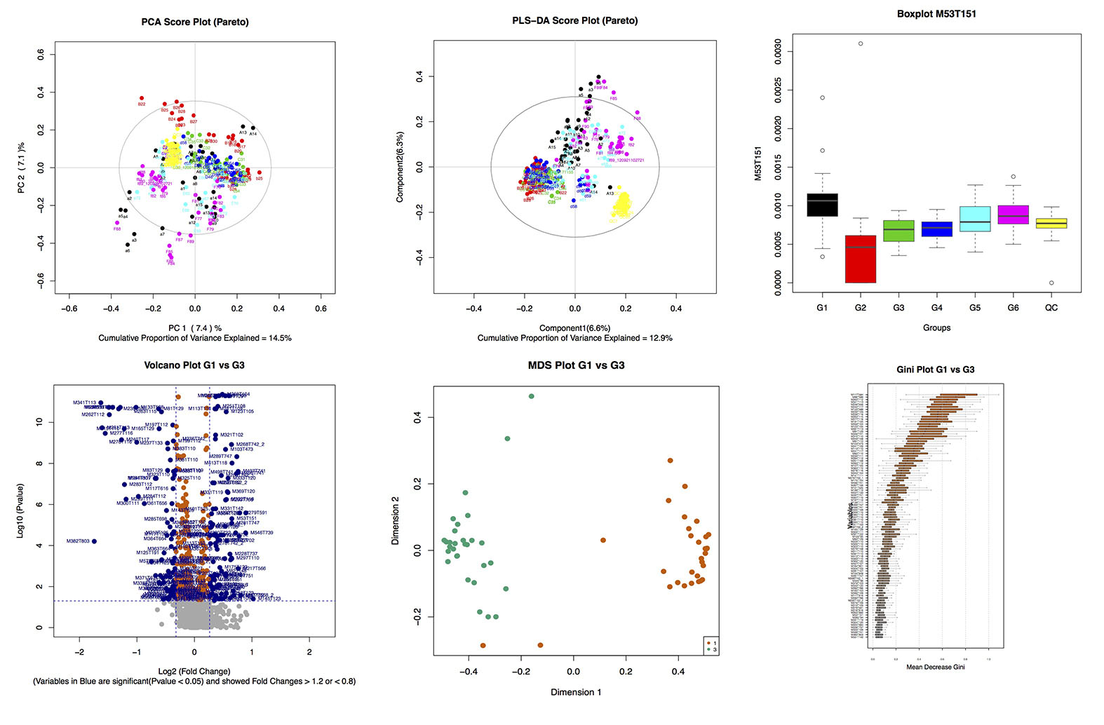
## Results of statistic analysis (statAnalysis)
- __The output file: __
```
statTarget -- statAnalysis
-- PCA_Data_Pareto # Principal Component Analysis
-- PLS_DA_Pareto # Partial least squares Discriminant Analysis
-- Univariate# The RSD analysis
----- BoxPlot
----- Fold_Changes
----- Mann-Whitney_Tests # For non-normally distributed variables
----- oddratio # odd ratio
----- Pvalues # Intergation pvalues from Welch_test and MWT_test
----- RForest # Random Forest
----- ROC # receiver operating characteristic curve
----- Shapiro_Tests
----- Significant_Variables # The Peaks with P-value < 0.05
----- Volcano_Plots
----- WelchTest # For normally distributed variables
```
- **The Figures:**
- **The status log (Example data):**
```
#############################
# Shift Correction function #
#############################
Data File Checking Start..., Time: Thu Jan 5 18:58:09 2017
217 Pheno Samples vs 218 Profile samples
The Pheno samples list (*NA, missing data from the Profile File)
[1] "QC1" "QC2" "QC3" "QC4"
[5] "QC5" "A1" "A2" "A3"
[9] "A4" "A5" "A6" "A7"
[13] "A8" "A9" "A10" "QC6"
[17] "A11" "A12" "A13" "A14"
[21] "A15" "B16" "B17" "B18"
[25] "B19" "B20" "QC7" "B21"
[29] "B22" "B23" "B24" "B25"
[33] "B26" "B27" "B28" "B29"
[37] "B30" "QC8" "C31" "C32"
[41] "C33" "C34" "C35" "QC9"
[45] "QC10" "QC11" "QC12" "QC13"
[49] "C36_120918171155" "C37" "C38" "C39"
[53] "C40" "QC14" "C41" "C42"
[57] "C43" "C44" "C45" "D46"
[61] "D47" "D48" "D49" "D50"
[65] "QC15" "D51" "D52" "D53"
[69] "D54" "D55" "D56" "D57"
[73] "D58" "D59" "D60" "QC16"
[77] "E61" "E62" "E63" "E64"
[81] "E65" "E66" "E67" "E68"
[85] "E69" "E70" "QC17" "E71"
[89] "E72" "E73" "E74" "E75"
[93] "F76" "F77" "F78" "F79"
[97] "F80" "QC18" "F81" "F82"
[101] "F83" "F84" "F85" "F86"
[105] "F87" "F88" "F89" "F90"
[109] "QC19" "QC20" "QC21" "QC22"
[113] "QC23" "QC24" "a1" "a2"
[117] "a3" "a4" "a5" "a6"
[121] "a7" "a8" "a9" "a10"
[125] "QC25" "a11" "a12" "a13"
[129] "a14" "a15" "b16" "b18"
[133] "b19" "b20" "QC26" "b21"
[137] "b22" "b23" "b24" "b25"
[141] "b26" "b27" "b28" "b29"
[145] "b30" "QC27" "c31" "c32"
[149] "c33" "c34" "c35" "QC28"
[153] "QC29" "QC31" "QC32" "c36"
[157] "c37" "c38" "c39" "c40"
[161] "QC33" "c41" "c42" "c43"
[165] "c44" "c45" "d46" "d47"
[169] "d48" "d49" "d50" "QC34"
[173] "d51" "d52" "d53" "d54"
[177] "d55" "d56" "d57" "d58"
[181] "d59" "d60" "QC35" "e61"
[185] "e62" "e63" "e64" "e65"
[189] "e66" "e67" "e68" "e69"
[193] "e70" "QC36" "e71" "e72"
[197] "e73" "e74" "e75" "f76"
[201] "f77" "f78" "f79" "f80"
[205] "QC37" "f81" "f82" "f83"
[209] "f84" "f85" "f86" "f87"
[213] "f88" "f89_120921102721" "f90" "QC38"
[217] "QC39"
Warning: The sample size in Profile File is larger than Pheno File!
Pheno information:
Class No.
1 1 30
2 2 29
3 3 30
4 4 30
5 5 30
6 6 30
7 QC 38
Batch No.
1 1 108
2 2 109
Profile information:
No.
QC and samples 218
Metabolites 1312
statTarget: shiftCor start...Time: Thu Jan 5 18:58:11 2017
Step 1: Evaluation of missing value...
The number of NA value in Data Profile before QC-RLSC: 2280
The number of variables including 80 % of missing value : 3
Step 2: Imputation start...
The number of NA value in Data Profile after the initial imputation: 0
Imputation Finished!
Step 3: QC-RLSC Start... Time: Thu Jan 5 18:58:12 2017
Warning: The QCspan was set at '0'.
The GCV was used to avoid overfitting the observed data
|===============================================================================| 100%
High-resolution images output...
Calculation of CV distribution of raw peaks (QC)...
CV<5% CV<10% CV<15% CV<20% CV<25% CV<30% CV<35% CV<40%
Batch_1 0.6875477 7.944996 23.98778 37.58594 46.98243 54.39267 61.19175 67.99083
Batch_2 4.0488923 25.821238 45.76012 57.44843 64.40031 70.51184 76.39419 80.29030
Total 0.3819710 6.722689 21.08480 33.38426 44.38503 51.87166 59.20550 64.55309
CV<45% CV<50% CV<55% CV<60% CV<65% CV<70% CV<75% CV<80% CV<85%
Batch_1 72.80367 77.92208 80.97785 84.11001 87.16578 88.69366 89.45760 90.67991 91.59664
Batch_2 83.34607 86.40183 88.31169 90.52712 92.58976 93.43010 94.42322 95.64553 96.18029
Total 69.36593 74.56073 78.53323 81.51261 82.96409 85.10313 87.39496 89.53400 91.36746
CV<90% CV<95% CV<100%
Batch_1 92.66616 93.35371 94.57601
Batch_2 96.48587 97.17341 97.40260
Total 92.89534 94.27044 94.95798
Calculation of CV distribution of corrected peaks (QC)...
CV<5% CV<10% CV<15% CV<20% CV<25% CV<30% CV<35% CV<40% CV<45%
Batch_1 18.25821 45.98930 64.40031 72.72727 78.45684 83.72804 86.17265 88.54087 89.76318
Batch_2 20.24446 51.48969 68.06723 78.22765 84.56837 88.23529 90.75630 92.36058 93.50649
Total 15.73720 44.46142 64.62949 73.18564 80.36669 84.79756 87.31856 88.69366 89.68678
CV<50% CV<55% CV<60% CV<65% CV<70% CV<75% CV<80% CV<85% CV<90%
Batch_1 91.06188 91.90222 92.58976 93.04813 93.43010 94.04125 94.65241 95.11077 95.56914
Batch_2 94.11765 94.88159 95.49274 96.18029 96.63866 96.86784 97.09702 97.40260 97.70817
Total 90.75630 91.97861 93.20092 93.96486 94.57601 95.33995 95.87471 96.10390 96.63866
CV<95% CV<100%
Batch_1 95.95111 96.02750
Batch_2 98.09015 98.31933
Total 96.71505 97.09702
Correction Finished! Time: Thu Jan 5 19:00:51 2017
```
## Results of statistic analysis (statAnalysis)
- __The output file: __
```
statTarget -- statAnalysis
-- PCA_Data_Pareto # Principal Component Analysis
-- PLS_DA_Pareto # Partial least squares Discriminant Analysis
-- Univariate# The RSD analysis
----- BoxPlot
----- Fold_Changes
----- Mann-Whitney_Tests # For non-normally distributed variables
----- oddratio # odd ratio
----- Pvalues # Intergation pvalues from Welch_test and MWT_test
----- RForest # Random Forest
----- ROC # receiver operating characteristic curve
----- Shapiro_Tests
----- Significant_Variables # The Peaks with P-value < 0.05
----- Volcano_Plots
----- WelchTest # For normally distributed variables
```
- **The Figures:**
 - **The status log (Example data):**
```
#################################
# Statistical Analysis function #
#################################
statTarget: statistical analysis start... Time: Fri Jan 6 11:57:48 2017
Step 1: Evaluation of missing value...
The number of NA value in Data Profile: 0
The number of variables including 80 % of missing value : 0
Step 2: Imputation start... Time: Fri Jan 6 11:57:50 2017
The number of NA value in Data Profile after the initialimputation: 0
Imputation Finished!
Step 3: Statistic Summary Start... Time: Fri Jan 6 11:57:50 2017
Step 4: Glog PCA-PLSDA start... Time: Fri Jan 6 11:58:19 2017
PCA Model Summary
217 samples x 1309 variables
Variance Explained of PCA Model:
PC1 PC2 PC3 PC4 PC5 PC6
Standard deviation 0.1471269 0.143504 0.1286476 0.1217399 0.1087545 0.1029451
Proportion of Variance 0.0743800 0.070770 0.0568700 0.0509300 0.0406400 0.0364200
Cumulative Proportion 0.0743800 0.145150 0.2020200 0.2529500 0.2935900 0.3300100
PC7 PC8 PC9 PC10 PC11 PC12
Standard deviation 0.09463045 0.09204723 0.08859019 0.08179698 0.07815861 0.07343806
Proportion of Variance 0.03077000 0.02911000 0.02697000 0.02299000 0.02099000 0.01853000
Cumulative Proportion 0.36078000 0.38989000 0.41686000 0.43985000 0.46085000 0.47938000
PC13 PC14 PC15 PC16 PC17 PC18
Standard deviation 0.06927193 0.06884729 0.06481461 0.06338068 0.0625105 0.05918608
Proportion of Variance 0.01649000 0.01629000 0.01444000 0.01380000 0.0134300 0.01204000
Cumulative Proportion 0.49587000 0.51216000 0.52659000 0.54040000 0.5538200 0.56586000
PC19 PC20 PC21 PC22 PC23 PC24
Standard deviation 0.05852846 0.0565814 0.05494036 0.05354714 0.05199812 0.0514794
Proportion of Variance 0.01177000 0.0110000 0.01037000 0.00985000 0.00929000 0.0091100
Cumulative Proportion 0.57763000 0.5886300 0.59901000 0.60886000 0.61815000 0.6272600
PC25 PC26 PC27 PC28 PC29 PC30
Standard deviation 0.05023623 0.05002373 0.04918839 0.04848824 0.04719809 0.04592107
Proportion of Variance 0.00867000 0.00860000 0.00831000 0.00808000 0.00765000 0.00725000
Cumulative Proportion 0.63593000 0.64453000 0.65284000 0.66092000 0.66858000 0.67582000
PC31 PC32 PC33 PC34 PC35 PC36
Standard deviation 0.04495383 0.04433005 0.043467 0.04273003 0.04211339 0.04168549
Proportion of Variance 0.00694000 0.00675000 0.006490 0.00627000 0.00609000 0.00597000
Cumulative Proportion 0.68277000 0.68952000 0.696010 0.70229000 0.70838000 0.71435000
PC37 PC38 PC39 PC40 PC41 PC42
Standard deviation 0.04074753 0.0399799 0.03970366 0.0395391 0.03887607 0.03829039
Proportion of Variance 0.00571000 0.0054900 0.00542000 0.0053700 0.00519000 0.00504000
Cumulative Proportion 0.72006000 0.7255500 0.73097000 0.7363400 0.74153000 0.74657000
PC43 PC44 PC45 PC46 PC47 PC48
Standard deviation 0.03757011 0.03717074 0.03680406 0.03627876 0.03578231 0.03561238
Proportion of Variance 0.00485000 0.00475000 0.00465000 0.00452000 0.00440000 0.00436000
Cumulative Proportion 0.75142000 0.75617000 0.76082000 0.76535000 0.76975000 0.77410000
PC49 PC50 PC51 PC52 PC53 PC54
Standard deviation 0.03500362 0.03466778 0.03451624 0.03404736 0.03367672 0.03328364
Proportion of Variance 0.00421000 0.00413000 0.00409000 0.00398000 0.00390000 0.00381000
Cumulative Proportion 0.77831000 0.78244000 0.78654000 0.79052000 0.79442000 0.79822000
PC55 PC56 PC57 PC58 PC59 PC60
Standard deviation 0.0329035 0.03283489 0.03263074 0.03220013 0.03174905 0.03127306
Proportion of Variance 0.0037200 0.00370000 0.00366000 0.00356000 0.00346000 0.00336000
Cumulative Proportion 0.8019400 0.80565000 0.80931000 0.81287000 0.81634000 0.81970000
PC61 PC62 PC63 PC64 PC65 PC66
Standard deviation 0.03099456 0.03067399 0.03047579 0.03027017 0.0299977 0.0293092
Proportion of Variance 0.00330000 0.00323000 0.00319000 0.00315000 0.0030900 0.0029500
Cumulative Proportion 0.82300000 0.82623000 0.82942000 0.83257000 0.8356600 0.8386100
PC67 PC68 PC69 PC70 PC71 PC72
Standard deviation 0.02910743 0.02891644 0.02871973 0.02851117 0.0284027 0.02802608
Proportion of Variance 0.00291000 0.00287000 0.00283000 0.00279000 0.0027700 0.00270000
Cumulative Proportion 0.84153000 0.84440000 0.84723000 0.85003000 0.8528000 0.85550000
PC73 PC74 PC75 PC76 PC77 PC78
Standard deviation 0.02767845 0.0274821 0.02707466 0.0270495 0.02689331 0.02669644
Proportion of Variance 0.00263000 0.0026000 0.00252000 0.0025100 0.00249000 0.00245000
Cumulative Proportion 0.85813000 0.8607300 0.86325000 0.8657600 0.86824000 0.87069000
PC79 PC80 PC81 PC82 PC83 PC84
Standard deviation 0.02641874 0.02597847 0.02569734 0.02537066 0.0252014 0.02514993
Proportion of Variance 0.00240000 0.00232000 0.00227000 0.00221000 0.0021800 0.00217000
Cumulative Proportion 0.87309000 0.87541000 0.87768000 0.87989000 0.8820700 0.88425000
PC85 PC86 PC87 PC88 PC89 PC90
Standard deviation 0.02505431 0.02457329 0.02445747 0.02427666 0.0240513 0.02389179
Proportion of Variance 0.00216000 0.00207000 0.00206000 0.00203000 0.0019900 0.00196000
Cumulative Proportion 0.88641000 0.88848000 0.89054000 0.89256000 0.8945500 0.89651000
PC91 PC92 PC93 PC94 PC95 PC96
Standard deviation 0.02381883 0.02338754 0.02322625 0.02314694 0.02290039 0.02280068
Proportion of Variance 0.00195000 0.00188000 0.00185000 0.00184000 0.00180000 0.00179000
Cumulative Proportion 0.89846000 0.90034000 0.90219000 0.90403000 0.90584000 0.90762000
PC97 PC98 PC99 PC100 PC101 PC102
Standard deviation 0.02259418 0.02254316 0.02231249 0.02210274 0.02203839 0.0219603
Proportion of Variance 0.00175000 0.00175000 0.00171000 0.00168000 0.00167000 0.0016600
Cumulative Proportion 0.90938000 0.91112000 0.91283000 0.91451000 0.91618000 0.9178400
PC103 PC104 PC105 PC106 PC107 PC108
Standard deviation 0.02173771 0.02144804 0.02114322 0.02103189 0.02086914 0.02065242
Proportion of Variance 0.00162000 0.00158000 0.00154000 0.00152000 0.00150000 0.00147000
Cumulative Proportion 0.91946000 0.92104000 0.92258000 0.92410000 0.92560000 0.92706000
PC109 PC110 PC111 PC112 PC113 PC114
Standard deviation 0.02033067 0.02023229 0.02004202 0.01989872 0.01975983 0.01957412
Proportion of Variance 0.00142000 0.00141000 0.00138000 0.00136000 0.00134000 0.00132000
Cumulative Proportion 0.92848000 0.92989000 0.93127000 0.93263000 0.93397000 0.93529000
PC115 PC116 PC117 PC118 PC119 PC120
Standard deviation 0.01944685 0.01934141 0.01919089 0.01906135 0.01896053 0.01881113
Proportion of Variance 0.00130000 0.00129000 0.00127000 0.00125000 0.00124000 0.00122000
Cumulative Proportion 0.93659000 0.93787000 0.93914000 0.94039000 0.94162000 0.94284000
PC121 PC122 PC123 PC124 PC125 PC126
Standard deviation 0.0187546 0.01861762 0.01844026 0.01822854 0.01801426 0.01786499
Proportion of Variance 0.0012100 0.00119000 0.00117000 0.00114000 0.00112000 0.00110000
Cumulative Proportion 0.9440500 0.94524000 0.94641000 0.94755000 0.94866000 0.94976000
PC127 PC128 PC129 PC130 PC131 PC132
Standard deviation 0.01785116 0.01775044 0.01756618 0.01746211 0.01721473 0.01709386
Proportion of Variance 0.00110000 0.00108000 0.00106000 0.00105000 0.00102000 0.00100000
Cumulative Proportion 0.95086000 0.95194000 0.95300000 0.95405000 0.95506000 0.95607000
PC133 PC134 PC135 PC136 PC137 PC138
Standard deviation 0.01705175 0.01684786 0.01671747 0.01664932 0.01648871 0.01640131
Proportion of Variance 0.00100000 0.00098000 0.00096000 0.00095000 0.00093000 0.00092000
Cumulative Proportion 0.95707000 0.95804000 0.95900000 0.95996000 0.96089000 0.96181000
PC139 PC140 PC141 PC142 PC143 PC144
Standard deviation 0.01632371 0.01600625 0.01580221 0.01571107 0.01562155 0.0155936
Proportion of Variance 0.00092000 0.00088000 0.00086000 0.00085000 0.00084000 0.0008400
Cumulative Proportion 0.96273000 0.96361000 0.96447000 0.96532000 0.96616000 0.9669900
PC145 PC146 PC147 PC148 PC149 PC150
Standard deviation 0.01537886 0.0152965 0.01517045 0.01506012 0.01501493 0.014774
Proportion of Variance 0.00081000 0.0008000 0.00079000 0.00078000 0.00077000 0.000750
Cumulative Proportion 0.96780000 0.9686100 0.96940000 0.97018000 0.97095000 0.971700
PC151 PC152 PC153 PC154 PC155 PC156
Standard deviation 0.01463149 0.0144876 0.01434792 0.01433986 0.01424448 0.01412483
Proportion of Variance 0.00074000 0.0007200 0.00071000 0.00071000 0.00070000 0.00069000
Cumulative Proportion 0.97244000 0.9731600 0.97387000 0.97457000 0.97527000 0.97596000
PC157 PC158 PC159 PC160 PC161 PC162
Standard deviation 0.01410833 0.01396131 0.01392313 0.01371741 0.01365028 0.01356903
Proportion of Variance 0.00068000 0.00067000 0.00067000 0.00065000 0.00064000 0.00063000
Cumulative Proportion 0.97664000 0.97731000 0.97798000 0.97862000 0.97926000 0.97990000
PC163 PC164 PC165 PC166 PC167 PC168
Standard deviation 0.01349251 0.01332544 0.01327065 0.01325211 0.01294927 0.01286386
Proportion of Variance 0.00063000 0.00061000 0.00061000 0.00060000 0.00058000 0.00057000
Cumulative Proportion 0.98052000 0.98113000 0.98174000 0.98234000 0.98292000 0.98349000
PC169 PC170 PC171 PC172 PC173 PC174
Standard deviation 0.01276056 0.01258496 0.01257078 0.01251062 0.01231667 0.01228647
Proportion of Variance 0.00056000 0.00054000 0.00054000 0.00054000 0.00052000 0.00052000
Cumulative Proportion 0.98404000 0.98459000 0.98513000 0.98567000 0.98619000 0.98671000
PC175 PC176 PC177 PC178 PC179 PC180
Standard deviation 0.01217565 0.01199646 0.01196251 0.01171993 0.01152939 0.01141553
Proportion of Variance 0.00051000 0.00049000 0.00049000 0.00047000 0.00046000 0.00045000
Cumulative Proportion 0.98722000 0.98771000 0.98821000 0.98868000 0.98913000 0.98958000
PC181 PC182 PC183 PC184 PC185 PC186
Standard deviation 0.01128977 0.01124502 0.0110693 0.01099837 0.01089239 0.01081447
Proportion of Variance 0.00044000 0.00043000 0.0004200 0.00042000 0.00041000 0.00040000
Cumulative Proportion 0.99002000 0.99045000 0.9908800 0.99129000 0.99170000 0.99210000
PC187 PC188 PC189 PC190 PC191 PC192
Standard deviation 0.01072824 0.01050272 0.01043874 0.01033548 0.01013789 0.01006607
Proportion of Variance 0.00040000 0.00038000 0.00037000 0.00037000 0.00035000 0.00035000
Cumulative Proportion 0.99250000 0.99288000 0.99325000 0.99362000 0.99397000 0.99432000
PC193 PC194 PC195 PC196 PC197
Standard deviation 0.009888063 0.009794131 0.009684863 0.009511312 0.009457666
Proportion of Variance 0.000340000 0.000330000 0.000320000 0.000310000 0.000310000
Cumulative Proportion 0.994650000 0.994980000 0.995310000 0.995620000 0.995920000
PC198 PC199 PC200 PC201 PC202
Standard deviation 0.009313158 0.009225365 0.009156228 0.008910202 0.00886853
Proportion of Variance 0.000300000 0.000290000 0.000290000 0.000270000 0.00027000
Cumulative Proportion 0.996220000 0.996520000 0.996800000 0.997080000 0.99735000
PC203 PC204 PC205 PC206 PC207
Standard deviation 0.008698389 0.008673122 0.008489401 0.008365039 0.00825881
Proportion of Variance 0.000260000 0.000260000 0.000250000 0.000240000 0.00023000
Cumulative Proportion 0.997610000 0.997860000 0.998110000 0.998350000 0.99859000
PC208 PC209 PC210 PC211 PC212
Standard deviation 0.008037357 0.007981711 0.007688713 0.007528352 0.007244244
Proportion of Variance 0.000220000 0.000220000 0.000200000 0.000190000 0.000180000
Cumulative Proportion 0.998810000 0.999030000 0.999230000 0.999430000 0.999610000
PC213 PC214 PC215 PC216 PC217
Standard deviation 0.007139559 0.005997918 0.004271462 0.00305905 1.082174e-16
Proportion of Variance 0.000180000 0.000120000 0.000060000 0.00003000 0.000000e+00
Cumulative Proportion 0.999780000 0.999910000 0.999970000 1.00000000 1.000000e+00
The following observations are calculated as outliers:
[1] "a3" "a6" "B22" "F84" "F86" "F88"
PLS(-DA) Two Component Model Summary
217 samples x 1309 variables
Cumulative Proportion of Variance Explained: R2X(cum) = 12.86179%
Cumulative Proportion of Response(s):
Y1 Y2 Y3 Y4 Y5 Y6 Y7
R2Y(cum) 0.1969126 0.2318528 0.1584459 0.10698318 0.020843739 0.3107075 0.7235089
Q2Y(cum) 0.1341826 0.1893128 0.1428475 0.08146868 0.007217958 0.2840960 0.6905388
Warning: More than two groups, permutation test skipped!
Warning: VIP was only implemented for the single-response model!
Step 5: Univariate Test Start...! Time: Fri Jan 6 11:58:33 2017
P-value Calculating...
*P-value was adjusted using Benjamini-Hochberg Method
Odd.Ratio Calculating...
ROC Calculating...
*Group.G1 Vs. Group.G2
|===============================================================================| 100%
*Group.G1 Vs. Group.G3
|===============================================================================| 100%
*Group.G1 Vs. Group.G4
|===============================================================================| 100%
*Group.G1 Vs. Group.G5
|===============================================================================| 100%
*Group.G1 Vs. Group.G6
|===============================================================================| 100%
*Group.G1 Vs. Group.QC
|===============================================================================| 100%
*Group.G2 Vs. Group.G3
|===============================================================================| 100%
*Group.G2 Vs. Group.G4
|===============================================================================| 100%
*Group.G2 Vs. Group.G5
|===============================================================================| 100%
*Group.G2 Vs. Group.G6
|===============================================================================| 100%
*Group.G2 Vs. Group.QC
|===============================================================================| 100%
*Group.G3 Vs. Group.G4
|===============================================================================| 100%
*Group.G3 Vs. Group.G5
|===============================================================================| 100%
*Group.G3 Vs. Group.G6
|===============================================================================| 100%
*Group.G3 Vs. Group.QC
|===============================================================================| 100%
*Group.G4 Vs. Group.G5
|===============================================================================| 100%
*Group.G4 Vs. Group.G6
|===============================================================================| 100%
*Group.G4 Vs. Group.QC
|===============================================================================| 100%
*Group.G5 Vs. Group.G6
|===============================================================================| 100%
*Group.G5 Vs. Group.QC
|===============================================================================| 100%
*Group.G6 Vs. Group.QC
|===============================================================================| 100%
RandomForest Calculating...
*Group.G1 Vs. Group.G2
|===============================================================================| 100%
*Group.G1 Vs. Group.G3
|===============================================================================| 100%
*Group.G1 Vs. Group.G4
|===============================================================================| 100%
*Group.G1 Vs. Group.G5
|===============================================================================| 100%
*Group.G1 Vs. Group.G6
|===============================================================================| 100%
*Group.G1 Vs. Group.QC
|===============================================================================| 100%
*Group.G2 Vs. Group.G3
|===============================================================================| 100%
*Group.G2 Vs. Group.G4
|===============================================================================| 100%
*Group.G2 Vs. Group.G5
|===============================================================================| 100%
*Group.G2 Vs. Group.G6
|===============================================================================| 100%
*Group.G2 Vs. Group.QC
|===============================================================================| 100%
*Group.G3 Vs. Group.G4
|===============================================================================| 100%
*Group.G3 Vs. Group.G5
|===============================================================================| 100%
*Group.G3 Vs. Group.G6
|===============================================================================| 100%
*Group.G3 Vs. Group.QC
|===============================================================================| 100%
*Group.G4 Vs. Group.G5
|===============================================================================| 100%
*Group.G4 Vs. Group.G6
|===============================================================================| 100%
*Group.G4 Vs. Group.QC
|===============================================================================| 100%
*Group.G5 Vs. Group.G6
|===============================================================================| 100%
*Group.G5 Vs. Group.QC
|===============================================================================| 100%
*Group.G6 Vs. Group.QC
|===============================================================================| 100%
Volcano Plot and Box Plot Output...
Statistical Analysis Finished! Time: Fri Jan 6 12:42:04 2017
```
# Session info
Here is the output of sessionInfo on the system on which this document was compiled:
```{r sessionInfo, eval = TRUE, echo = TRUE}
sessionInfo()
```
# References
Dunn, W.B., et al.,Procedures for large-scale metabolic profiling of
serum and plasma using gas chromatography and liquid chromatography coupled
to mass spectrometry. Nature Protocols 2011, 6, 1060.
Luan H., LC-MS-Based Urinary Metabolite Signatures in Idiopathic
Parkinson's Disease. J Proteome Res., 2015, 14,467.
Luan H., Non-targeted metabolomics and lipidomics LC-MS data
from maternal plasma of 180 healthy pregnant women. GigaScience 2015 4:16
- **The status log (Example data):**
```
#################################
# Statistical Analysis function #
#################################
statTarget: statistical analysis start... Time: Fri Jan 6 11:57:48 2017
Step 1: Evaluation of missing value...
The number of NA value in Data Profile: 0
The number of variables including 80 % of missing value : 0
Step 2: Imputation start... Time: Fri Jan 6 11:57:50 2017
The number of NA value in Data Profile after the initialimputation: 0
Imputation Finished!
Step 3: Statistic Summary Start... Time: Fri Jan 6 11:57:50 2017
Step 4: Glog PCA-PLSDA start... Time: Fri Jan 6 11:58:19 2017
PCA Model Summary
217 samples x 1309 variables
Variance Explained of PCA Model:
PC1 PC2 PC3 PC4 PC5 PC6
Standard deviation 0.1471269 0.143504 0.1286476 0.1217399 0.1087545 0.1029451
Proportion of Variance 0.0743800 0.070770 0.0568700 0.0509300 0.0406400 0.0364200
Cumulative Proportion 0.0743800 0.145150 0.2020200 0.2529500 0.2935900 0.3300100
PC7 PC8 PC9 PC10 PC11 PC12
Standard deviation 0.09463045 0.09204723 0.08859019 0.08179698 0.07815861 0.07343806
Proportion of Variance 0.03077000 0.02911000 0.02697000 0.02299000 0.02099000 0.01853000
Cumulative Proportion 0.36078000 0.38989000 0.41686000 0.43985000 0.46085000 0.47938000
PC13 PC14 PC15 PC16 PC17 PC18
Standard deviation 0.06927193 0.06884729 0.06481461 0.06338068 0.0625105 0.05918608
Proportion of Variance 0.01649000 0.01629000 0.01444000 0.01380000 0.0134300 0.01204000
Cumulative Proportion 0.49587000 0.51216000 0.52659000 0.54040000 0.5538200 0.56586000
PC19 PC20 PC21 PC22 PC23 PC24
Standard deviation 0.05852846 0.0565814 0.05494036 0.05354714 0.05199812 0.0514794
Proportion of Variance 0.01177000 0.0110000 0.01037000 0.00985000 0.00929000 0.0091100
Cumulative Proportion 0.57763000 0.5886300 0.59901000 0.60886000 0.61815000 0.6272600
PC25 PC26 PC27 PC28 PC29 PC30
Standard deviation 0.05023623 0.05002373 0.04918839 0.04848824 0.04719809 0.04592107
Proportion of Variance 0.00867000 0.00860000 0.00831000 0.00808000 0.00765000 0.00725000
Cumulative Proportion 0.63593000 0.64453000 0.65284000 0.66092000 0.66858000 0.67582000
PC31 PC32 PC33 PC34 PC35 PC36
Standard deviation 0.04495383 0.04433005 0.043467 0.04273003 0.04211339 0.04168549
Proportion of Variance 0.00694000 0.00675000 0.006490 0.00627000 0.00609000 0.00597000
Cumulative Proportion 0.68277000 0.68952000 0.696010 0.70229000 0.70838000 0.71435000
PC37 PC38 PC39 PC40 PC41 PC42
Standard deviation 0.04074753 0.0399799 0.03970366 0.0395391 0.03887607 0.03829039
Proportion of Variance 0.00571000 0.0054900 0.00542000 0.0053700 0.00519000 0.00504000
Cumulative Proportion 0.72006000 0.7255500 0.73097000 0.7363400 0.74153000 0.74657000
PC43 PC44 PC45 PC46 PC47 PC48
Standard deviation 0.03757011 0.03717074 0.03680406 0.03627876 0.03578231 0.03561238
Proportion of Variance 0.00485000 0.00475000 0.00465000 0.00452000 0.00440000 0.00436000
Cumulative Proportion 0.75142000 0.75617000 0.76082000 0.76535000 0.76975000 0.77410000
PC49 PC50 PC51 PC52 PC53 PC54
Standard deviation 0.03500362 0.03466778 0.03451624 0.03404736 0.03367672 0.03328364
Proportion of Variance 0.00421000 0.00413000 0.00409000 0.00398000 0.00390000 0.00381000
Cumulative Proportion 0.77831000 0.78244000 0.78654000 0.79052000 0.79442000 0.79822000
PC55 PC56 PC57 PC58 PC59 PC60
Standard deviation 0.0329035 0.03283489 0.03263074 0.03220013 0.03174905 0.03127306
Proportion of Variance 0.0037200 0.00370000 0.00366000 0.00356000 0.00346000 0.00336000
Cumulative Proportion 0.8019400 0.80565000 0.80931000 0.81287000 0.81634000 0.81970000
PC61 PC62 PC63 PC64 PC65 PC66
Standard deviation 0.03099456 0.03067399 0.03047579 0.03027017 0.0299977 0.0293092
Proportion of Variance 0.00330000 0.00323000 0.00319000 0.00315000 0.0030900 0.0029500
Cumulative Proportion 0.82300000 0.82623000 0.82942000 0.83257000 0.8356600 0.8386100
PC67 PC68 PC69 PC70 PC71 PC72
Standard deviation 0.02910743 0.02891644 0.02871973 0.02851117 0.0284027 0.02802608
Proportion of Variance 0.00291000 0.00287000 0.00283000 0.00279000 0.0027700 0.00270000
Cumulative Proportion 0.84153000 0.84440000 0.84723000 0.85003000 0.8528000 0.85550000
PC73 PC74 PC75 PC76 PC77 PC78
Standard deviation 0.02767845 0.0274821 0.02707466 0.0270495 0.02689331 0.02669644
Proportion of Variance 0.00263000 0.0026000 0.00252000 0.0025100 0.00249000 0.00245000
Cumulative Proportion 0.85813000 0.8607300 0.86325000 0.8657600 0.86824000 0.87069000
PC79 PC80 PC81 PC82 PC83 PC84
Standard deviation 0.02641874 0.02597847 0.02569734 0.02537066 0.0252014 0.02514993
Proportion of Variance 0.00240000 0.00232000 0.00227000 0.00221000 0.0021800 0.00217000
Cumulative Proportion 0.87309000 0.87541000 0.87768000 0.87989000 0.8820700 0.88425000
PC85 PC86 PC87 PC88 PC89 PC90
Standard deviation 0.02505431 0.02457329 0.02445747 0.02427666 0.0240513 0.02389179
Proportion of Variance 0.00216000 0.00207000 0.00206000 0.00203000 0.0019900 0.00196000
Cumulative Proportion 0.88641000 0.88848000 0.89054000 0.89256000 0.8945500 0.89651000
PC91 PC92 PC93 PC94 PC95 PC96
Standard deviation 0.02381883 0.02338754 0.02322625 0.02314694 0.02290039 0.02280068
Proportion of Variance 0.00195000 0.00188000 0.00185000 0.00184000 0.00180000 0.00179000
Cumulative Proportion 0.89846000 0.90034000 0.90219000 0.90403000 0.90584000 0.90762000
PC97 PC98 PC99 PC100 PC101 PC102
Standard deviation 0.02259418 0.02254316 0.02231249 0.02210274 0.02203839 0.0219603
Proportion of Variance 0.00175000 0.00175000 0.00171000 0.00168000 0.00167000 0.0016600
Cumulative Proportion 0.90938000 0.91112000 0.91283000 0.91451000 0.91618000 0.9178400
PC103 PC104 PC105 PC106 PC107 PC108
Standard deviation 0.02173771 0.02144804 0.02114322 0.02103189 0.02086914 0.02065242
Proportion of Variance 0.00162000 0.00158000 0.00154000 0.00152000 0.00150000 0.00147000
Cumulative Proportion 0.91946000 0.92104000 0.92258000 0.92410000 0.92560000 0.92706000
PC109 PC110 PC111 PC112 PC113 PC114
Standard deviation 0.02033067 0.02023229 0.02004202 0.01989872 0.01975983 0.01957412
Proportion of Variance 0.00142000 0.00141000 0.00138000 0.00136000 0.00134000 0.00132000
Cumulative Proportion 0.92848000 0.92989000 0.93127000 0.93263000 0.93397000 0.93529000
PC115 PC116 PC117 PC118 PC119 PC120
Standard deviation 0.01944685 0.01934141 0.01919089 0.01906135 0.01896053 0.01881113
Proportion of Variance 0.00130000 0.00129000 0.00127000 0.00125000 0.00124000 0.00122000
Cumulative Proportion 0.93659000 0.93787000 0.93914000 0.94039000 0.94162000 0.94284000
PC121 PC122 PC123 PC124 PC125 PC126
Standard deviation 0.0187546 0.01861762 0.01844026 0.01822854 0.01801426 0.01786499
Proportion of Variance 0.0012100 0.00119000 0.00117000 0.00114000 0.00112000 0.00110000
Cumulative Proportion 0.9440500 0.94524000 0.94641000 0.94755000 0.94866000 0.94976000
PC127 PC128 PC129 PC130 PC131 PC132
Standard deviation 0.01785116 0.01775044 0.01756618 0.01746211 0.01721473 0.01709386
Proportion of Variance 0.00110000 0.00108000 0.00106000 0.00105000 0.00102000 0.00100000
Cumulative Proportion 0.95086000 0.95194000 0.95300000 0.95405000 0.95506000 0.95607000
PC133 PC134 PC135 PC136 PC137 PC138
Standard deviation 0.01705175 0.01684786 0.01671747 0.01664932 0.01648871 0.01640131
Proportion of Variance 0.00100000 0.00098000 0.00096000 0.00095000 0.00093000 0.00092000
Cumulative Proportion 0.95707000 0.95804000 0.95900000 0.95996000 0.96089000 0.96181000
PC139 PC140 PC141 PC142 PC143 PC144
Standard deviation 0.01632371 0.01600625 0.01580221 0.01571107 0.01562155 0.0155936
Proportion of Variance 0.00092000 0.00088000 0.00086000 0.00085000 0.00084000 0.0008400
Cumulative Proportion 0.96273000 0.96361000 0.96447000 0.96532000 0.96616000 0.9669900
PC145 PC146 PC147 PC148 PC149 PC150
Standard deviation 0.01537886 0.0152965 0.01517045 0.01506012 0.01501493 0.014774
Proportion of Variance 0.00081000 0.0008000 0.00079000 0.00078000 0.00077000 0.000750
Cumulative Proportion 0.96780000 0.9686100 0.96940000 0.97018000 0.97095000 0.971700
PC151 PC152 PC153 PC154 PC155 PC156
Standard deviation 0.01463149 0.0144876 0.01434792 0.01433986 0.01424448 0.01412483
Proportion of Variance 0.00074000 0.0007200 0.00071000 0.00071000 0.00070000 0.00069000
Cumulative Proportion 0.97244000 0.9731600 0.97387000 0.97457000 0.97527000 0.97596000
PC157 PC158 PC159 PC160 PC161 PC162
Standard deviation 0.01410833 0.01396131 0.01392313 0.01371741 0.01365028 0.01356903
Proportion of Variance 0.00068000 0.00067000 0.00067000 0.00065000 0.00064000 0.00063000
Cumulative Proportion 0.97664000 0.97731000 0.97798000 0.97862000 0.97926000 0.97990000
PC163 PC164 PC165 PC166 PC167 PC168
Standard deviation 0.01349251 0.01332544 0.01327065 0.01325211 0.01294927 0.01286386
Proportion of Variance 0.00063000 0.00061000 0.00061000 0.00060000 0.00058000 0.00057000
Cumulative Proportion 0.98052000 0.98113000 0.98174000 0.98234000 0.98292000 0.98349000
PC169 PC170 PC171 PC172 PC173 PC174
Standard deviation 0.01276056 0.01258496 0.01257078 0.01251062 0.01231667 0.01228647
Proportion of Variance 0.00056000 0.00054000 0.00054000 0.00054000 0.00052000 0.00052000
Cumulative Proportion 0.98404000 0.98459000 0.98513000 0.98567000 0.98619000 0.98671000
PC175 PC176 PC177 PC178 PC179 PC180
Standard deviation 0.01217565 0.01199646 0.01196251 0.01171993 0.01152939 0.01141553
Proportion of Variance 0.00051000 0.00049000 0.00049000 0.00047000 0.00046000 0.00045000
Cumulative Proportion 0.98722000 0.98771000 0.98821000 0.98868000 0.98913000 0.98958000
PC181 PC182 PC183 PC184 PC185 PC186
Standard deviation 0.01128977 0.01124502 0.0110693 0.01099837 0.01089239 0.01081447
Proportion of Variance 0.00044000 0.00043000 0.0004200 0.00042000 0.00041000 0.00040000
Cumulative Proportion 0.99002000 0.99045000 0.9908800 0.99129000 0.99170000 0.99210000
PC187 PC188 PC189 PC190 PC191 PC192
Standard deviation 0.01072824 0.01050272 0.01043874 0.01033548 0.01013789 0.01006607
Proportion of Variance 0.00040000 0.00038000 0.00037000 0.00037000 0.00035000 0.00035000
Cumulative Proportion 0.99250000 0.99288000 0.99325000 0.99362000 0.99397000 0.99432000
PC193 PC194 PC195 PC196 PC197
Standard deviation 0.009888063 0.009794131 0.009684863 0.009511312 0.009457666
Proportion of Variance 0.000340000 0.000330000 0.000320000 0.000310000 0.000310000
Cumulative Proportion 0.994650000 0.994980000 0.995310000 0.995620000 0.995920000
PC198 PC199 PC200 PC201 PC202
Standard deviation 0.009313158 0.009225365 0.009156228 0.008910202 0.00886853
Proportion of Variance 0.000300000 0.000290000 0.000290000 0.000270000 0.00027000
Cumulative Proportion 0.996220000 0.996520000 0.996800000 0.997080000 0.99735000
PC203 PC204 PC205 PC206 PC207
Standard deviation 0.008698389 0.008673122 0.008489401 0.008365039 0.00825881
Proportion of Variance 0.000260000 0.000260000 0.000250000 0.000240000 0.00023000
Cumulative Proportion 0.997610000 0.997860000 0.998110000 0.998350000 0.99859000
PC208 PC209 PC210 PC211 PC212
Standard deviation 0.008037357 0.007981711 0.007688713 0.007528352 0.007244244
Proportion of Variance 0.000220000 0.000220000 0.000200000 0.000190000 0.000180000
Cumulative Proportion 0.998810000 0.999030000 0.999230000 0.999430000 0.999610000
PC213 PC214 PC215 PC216 PC217
Standard deviation 0.007139559 0.005997918 0.004271462 0.00305905 1.082174e-16
Proportion of Variance 0.000180000 0.000120000 0.000060000 0.00003000 0.000000e+00
Cumulative Proportion 0.999780000 0.999910000 0.999970000 1.00000000 1.000000e+00
The following observations are calculated as outliers:
[1] "a3" "a6" "B22" "F84" "F86" "F88"
PLS(-DA) Two Component Model Summary
217 samples x 1309 variables
Cumulative Proportion of Variance Explained: R2X(cum) = 12.86179%
Cumulative Proportion of Response(s):
Y1 Y2 Y3 Y4 Y5 Y6 Y7
R2Y(cum) 0.1969126 0.2318528 0.1584459 0.10698318 0.020843739 0.3107075 0.7235089
Q2Y(cum) 0.1341826 0.1893128 0.1428475 0.08146868 0.007217958 0.2840960 0.6905388
Warning: More than two groups, permutation test skipped!
Warning: VIP was only implemented for the single-response model!
Step 5: Univariate Test Start...! Time: Fri Jan 6 11:58:33 2017
P-value Calculating...
*P-value was adjusted using Benjamini-Hochberg Method
Odd.Ratio Calculating...
ROC Calculating...
*Group.G1 Vs. Group.G2
|===============================================================================| 100%
*Group.G1 Vs. Group.G3
|===============================================================================| 100%
*Group.G1 Vs. Group.G4
|===============================================================================| 100%
*Group.G1 Vs. Group.G5
|===============================================================================| 100%
*Group.G1 Vs. Group.G6
|===============================================================================| 100%
*Group.G1 Vs. Group.QC
|===============================================================================| 100%
*Group.G2 Vs. Group.G3
|===============================================================================| 100%
*Group.G2 Vs. Group.G4
|===============================================================================| 100%
*Group.G2 Vs. Group.G5
|===============================================================================| 100%
*Group.G2 Vs. Group.G6
|===============================================================================| 100%
*Group.G2 Vs. Group.QC
|===============================================================================| 100%
*Group.G3 Vs. Group.G4
|===============================================================================| 100%
*Group.G3 Vs. Group.G5
|===============================================================================| 100%
*Group.G3 Vs. Group.G6
|===============================================================================| 100%
*Group.G3 Vs. Group.QC
|===============================================================================| 100%
*Group.G4 Vs. Group.G5
|===============================================================================| 100%
*Group.G4 Vs. Group.G6
|===============================================================================| 100%
*Group.G4 Vs. Group.QC
|===============================================================================| 100%
*Group.G5 Vs. Group.G6
|===============================================================================| 100%
*Group.G5 Vs. Group.QC
|===============================================================================| 100%
*Group.G6 Vs. Group.QC
|===============================================================================| 100%
RandomForest Calculating...
*Group.G1 Vs. Group.G2
|===============================================================================| 100%
*Group.G1 Vs. Group.G3
|===============================================================================| 100%
*Group.G1 Vs. Group.G4
|===============================================================================| 100%
*Group.G1 Vs. Group.G5
|===============================================================================| 100%
*Group.G1 Vs. Group.G6
|===============================================================================| 100%
*Group.G1 Vs. Group.QC
|===============================================================================| 100%
*Group.G2 Vs. Group.G3
|===============================================================================| 100%
*Group.G2 Vs. Group.G4
|===============================================================================| 100%
*Group.G2 Vs. Group.G5
|===============================================================================| 100%
*Group.G2 Vs. Group.G6
|===============================================================================| 100%
*Group.G2 Vs. Group.QC
|===============================================================================| 100%
*Group.G3 Vs. Group.G4
|===============================================================================| 100%
*Group.G3 Vs. Group.G5
|===============================================================================| 100%
*Group.G3 Vs. Group.G6
|===============================================================================| 100%
*Group.G3 Vs. Group.QC
|===============================================================================| 100%
*Group.G4 Vs. Group.G5
|===============================================================================| 100%
*Group.G4 Vs. Group.G6
|===============================================================================| 100%
*Group.G4 Vs. Group.QC
|===============================================================================| 100%
*Group.G5 Vs. Group.G6
|===============================================================================| 100%
*Group.G5 Vs. Group.QC
|===============================================================================| 100%
*Group.G6 Vs. Group.QC
|===============================================================================| 100%
Volcano Plot and Box Plot Output...
Statistical Analysis Finished! Time: Fri Jan 6 12:42:04 2017
```
# Session info
Here is the output of sessionInfo on the system on which this document was compiled:
```{r sessionInfo, eval = TRUE, echo = TRUE}
sessionInfo()
```
# References
Dunn, W.B., et al.,Procedures for large-scale metabolic profiling of
serum and plasma using gas chromatography and liquid chromatography coupled
to mass spectrometry. Nature Protocols 2011, 6, 1060.
Luan H., LC-MS-Based Urinary Metabolite Signatures in Idiopathic
Parkinson's Disease. J Proteome Res., 2015, 14,467.
Luan H., Non-targeted metabolomics and lipidomics LC-MS data
from maternal plasma of 180 healthy pregnant women. GigaScience 2015 4:16